Tutorial : optical system for adapting two beams - paraxial system adapting two gaussian beams
Laser beam
Geometric optics is not sufficient to explain light emission by a laser. Electromagnetic theory with limit conditions given by spatial and phase stabilities after one round trip in the cavity impose that only specific waves can oscillate. They are called the transverse modes of the laser. In Gauss conditions, they are solutions of the Maxwell equation in isotropic media using the paraxial approximation :
 .
Among others, these waves depend on the mirrors shape and their relative positions. Different models exist depending on the cavity. The models pedict modes with different kinds of intensity distributions. If the mirrors have a rectangular symetry, Hermito gaussian modes may propagate. The amplitude of the Hermito Gaussian mode Hpq is given by :
.
Among others, these waves depend on the mirrors shape and their relative positions. Different models exist depending on the cavity. The models pedict modes with different kinds of intensity distributions. If the mirrors have a rectangular symetry, Hermito gaussian modes may propagate. The amplitude of the Hermito Gaussian mode Hpq is given by :
 .
.
 is an Hermite polynomial.
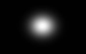
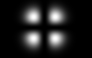
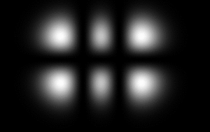
The intensity distribution of Hermito gaussian modes H00, H11, H21 and H22 are illustrated below.
is an Hermite polynomial.
The intensity distribution of Hermito gaussian modes H00, H11, H21 and H22 are illustrated below.
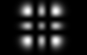
In cavities with a cylindrical symetry, Laguerre gaussian modes may propagate. The amplitude of the is given by the formula below :
 .
.
 is a Laguerre polynomial.
Among all the modes, the fundamental mode (common to Hermito gaussian and Laguerre Gaussian modes) is also called TEM00 mode or gaussian mode because its intensity distribution in a transverse plane XY perpendicular to the propagation has a gaussian shape. Its amplitude distribution is :
is a Laguerre polynomial.
Among all the modes, the fundamental mode (common to Hermito gaussian and Laguerre Gaussian modes) is also called TEM00 mode or gaussian mode because its intensity distribution in a transverse plane XY perpendicular to the propagation has a gaussian shape. Its amplitude distribution is :
 .
.
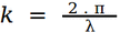 ,
,  ,
,  ,
,  ,
, 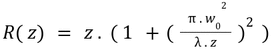 .
R(z) is the radius of curvature of the wave front at the distance z from the waist.
The intensity is:
.
R(z) is the radius of curvature of the wave front at the distance z from the waist.
The intensity is:
 .
.
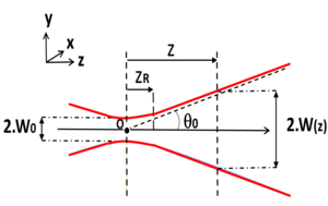
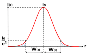 Whatever the transverse plane, the beam is commonly delimited by the circle for which the relative intensity is 1 / e2 and therefore containing 86,5% of the light power. This circle diameter is 2 .w(z) and is defined as the beam diameter at the considered position on the propagation axis. The beam diameter changes along the propagation axis and forms an hyperboloidic envelope . The beam half divergence is
 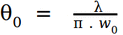 . The origin O of the propagation axis is taken on the waist where the beam cross section is the smallest.
The half diameter of the waist is w0.
The Rayleigh range defined by 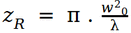 is a characteristic parameter of the beam.
if
is a characteristic parameter of the beam.
if  , the considered zone is commonly called the "near field " and
 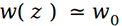 . The wavefront shape is rather flat.
if
. The wavefront shape is rather flat.
if  , the considered zone is commonly called the "far field" and
  . The beam is diverging and the wavefront is spherical and approximately centered on the waist center.
The fundamental mode is the less diverging mode and thus it has the highest spatial coherence. Therefore, most laser suppliers try to manufacture lasers emitting in the fundamental mode only.
In reality, laser beams can never be exactly gaussian, first because the involved theory is an approximation in the paraxial conditions, second because the cavity is not prefect (mirrors shape and positionning are not exactly as designed) or simply because the beam can not be fully cleaned and it is a combination of the gaussian mode with higher order modes. Whatever the beam, it has a waist (location where its cross section is the smallest) and a divergence which is necessarily larger than the divergence of the theoretical gaussian beam with the same waist radius.
. The beam is diverging and the wavefront is spherical and approximately centered on the waist center.
The fundamental mode is the less diverging mode and thus it has the highest spatial coherence. Therefore, most laser suppliers try to manufacture lasers emitting in the fundamental mode only.
In reality, laser beams can never be exactly gaussian, first because the involved theory is an approximation in the paraxial conditions, second because the cavity is not prefect (mirrors shape and positionning are not exactly as designed) or simply because the beam can not be fully cleaned and it is a combination of the gaussian mode with higher order modes. Whatever the beam, it has a waist (location where its cross section is the smallest) and a divergence which is necessarily larger than the divergence of the theoretical gaussian beam with the same waist radius.
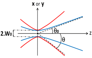 A simple way to modelize the propagation is then to consider the beam as an "embedded" gaussian beam with an hyperboloidic shape and which divergence is given by θ with
 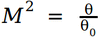 . The M2 factor (or "M-square" factor) is therefore larger than 1. The "embedded" gaussian beam parameters can be calculated using the fundamental mode formulas and replacing
  .
For example, the beam rayleigh range becomes
.
For example, the beam rayleigh range becomes 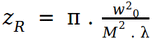 .
.
M2 can be specified smaller than 1.05 for relatively low power lasers and can achieve several dozens for high power lasers. Note that the concept of low or high power is strongly dependant on the technology. For example, Argon lasers can have low M2 (close to 1) with power in the range of 20 W while laser diodes are generally multimode at power of a few Watts and even less.
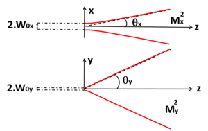 There are cases where the gain medium as well as the mirrors have a rectangular symetry as for instance in semiconductor lasers which gain medium is a parallelipipedic waveguide. The fundamental mode can then be modellized as gaussian in the XZ and YZ planes with different waist dimensions
 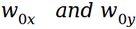 and different divergences
 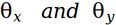 ....
For embedded gaussian beams, the "M-square" factors M2x and M2y are defined respectively in the XZ and YZ planes.
....
For embedded gaussian beams, the "M-square" factors M2x and M2y are defined respectively in the XZ and YZ planes.
Obviously, M2x and M2y can have different values. For example, high power laser diodes made of a single wave guide (emitting few Watts) have a thickness (in the range of hundred microns) very different from the height ( in the range of the micron) and thus the M2y corresponding to the vertical plane is close to 1 while M2x corresponding to the horizontal plane is much higher than 1. Note that all semiconductor lasers don't have astigmatism. For example VCSELs (Vertical Cavity Surface Emitting lasers) can emit beams with a cylindrical symetry.
Laser beam shaping
In many cases, laser beams can not be used directly without being transformed. For example, a collimated beam naturally emitted by a Nd:Yag laser for material drilling generally requests to be focused both to obtain the desired hole diameter and a higher brightness. Also, a collimated laser beam from an Argon laser can not be efficiently coupled into a fiber optics which core diameter is generally smaller. It needs to be adequately focused on the fiber entrance. A semiconductor laser beam is naturally diverging and has to be first collimated and secondly focused on the fiber entrance to be injected efficiently. These examples are only a few and there are many others.
A gaussian beam after an optical surface in the paraxial approximation can be calculated thanks to the ABCD matrix used for paraxial conjugation.
In paraxial conjugation,  =
=  X
X  where ABCD is the propagation matrix from a plane P1 to another plane P2.
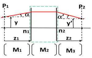 Considering an optical system between the two planes P1 and P2, the ABCD matrix is M3xM2xM1 where M1 is the propagation matrix from P1 to the primary principal plane, M2 is the propagation matrix through the optical system from the primary principal plane to the secondary principal plane and M3 is the propagation matrix from the secondary principal plane to P2.
M1 =  and M3 =
  .
n1 and n2 are the refraction indexes respectively before and after the optical system. z1 is the distance from P1 to the primary principal plane. z2 is the distance fom the secondary principal plane to P2.
The matrix M2 corresponding to the most common optical components are :
.
n1 and n2 are the refraction indexes respectively before and after the optical system. z1 is the distance from P1 to the primary principal plane. z2 is the distance fom the secondary principal plane to P2.
The matrix M2 corresponding to the most common optical components are :
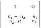 (spherical dioptrum),
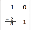 (spherical mirror),
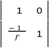 (thin lens)
The ABCD matrix can be used to calculate gaussian beams propagation. Let define Q(z) the complex curvature of the gaussian wave.
(thin lens)
The ABCD matrix can be used to calculate gaussian beams propagation. Let define Q(z) the complex curvature of the gaussian wave. 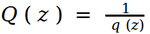 where .
The complex radii Q1(z) and Q2(z) respectively in P1 and P2 are corresponding by the formula :
(2)
where .
The complex radii Q1(z) and Q2(z) respectively in P1 and P2 are corresponding by the formula :
(2)  .
If z1 and z2 are the position of the waist respectively before and after the surface,
.
If z1 and z2 are the position of the waist respectively before and after the surface,  .
Q1(z) and Q2(z) are therefore imaginary.
.
Q1(z) and Q2(z) are therefore imaginary.
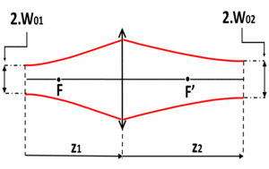 Knowing z1 and w01 (the waist position and its half diameter before the optical system), equation (2) allows to calculate z2 and w02 (the waist location and its half diameter after the optical system).
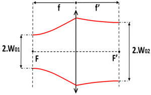 In the case of a thin lens, if the waist before the surface is located in the front focal plane, the waist after the lens is then located in the back focal plane and
 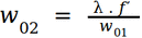 .
.
In these conditions, if w01 is small and thus the incident beam is diverging, w02 is large and the shaped beam has a small divergence. In the reversed situation where w01 is large and thus the incident beam is almost collimated, w02 is small and the transmitted beam is focused close to the back focal plane. Theses cases are quite similar to the cases encountered in geometric optics, the first one where the object is at the front focal plane and its conjugate is at infinity and the second one where the object is at infinity and its conjugate is at the back focal point.
For embedded gaussian beams, the calculation remains the same with :
 .
.
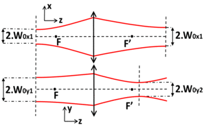 For elliptical beams, the calculations are realized similary but separately in each plane XZ and YZ plane with :
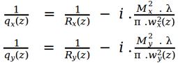 . Note that in general, the waists position after the optical system in the XZ and YZ plane may be different.
If the surface has no cylindrical symetry and is for example toroidal with Rx and Ry as radii respectively around X and Y axis, the transmission matrix M2x and M2y respectively in the XZ and YZ planes are :
M2x = 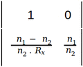 and M2y =
 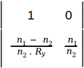 .
.