Tutorial : spherical aberration - spherical lens interfacing different media
Geometric aberrations
For optical systems which are not rigorously stigmatic or when Gauss conditions are not respected (which means that the angle with the axis of light rays coming from an object is large and/or the object is far from the axis), geometrical aberrations may appear. In this case, the image of a point is no more a point but a spot and therefore the image of a scene is blurred. Geometric aberrations are different from chromatic aberration which only appears in optical systems containing refractive components (like lenses for example) but can occure also under Gauss conditions. Chromatic aberration may blurr the image by generating images of the same object at different locations depending on the wavelength. Therefore, the chromatic aberration appears for objects illuminated with polychromatic sources as geometric aberration happens also with monochromatic sources. Note that only systems with a cylindrical symetry are considered in the following sections.
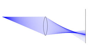
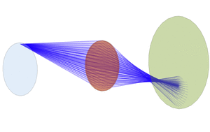
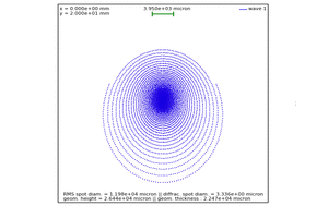 The pictures on the left illustrate the aberrations of a single spherical lens for an off-axis object on the Y axis (vertical). The furthest to the left picture represents the ray tracing in the YZ plane, that one in the middle is a ray tracing in perspective view and the most to the right one is the spot diagram obtained in the paraxial image plane.
Before describing aberrations, one must define the aperture of an optical system.
Aperture of an optical system
The aperture is supposed to be the only surface of the system stopping light rays. This surface can be in the object space, in the image space or in an intermediate space. In any case, it is possible to define the aperture in the object space: it is the conjugate of the aperture by the sub-system formed with the preceding components and used in the reverse way. Also, it is possible to define the aperture in the image space which is the conjugate of the aperture by the sub-system formed with the following components. The aperture in the object space enables to defines the solid angle inside which the rays are launched from the field(s). The aperture in the image space enables to eventually calculate the Wave Front Error and the associated parameters as well as the diffraction limit of the system. Note that in some cases, vignetting can appear. Indeed, some rays coming from off-xis objects may be stopped by another surface than the said aperture surface. This can affect the aberrations, limit the system resolution and create some shadows on the image. In general, one try to avoid vignetting and this case is not considered in the rest of the tutorial.
An optical system is represented in the pictures below with different aperture positions. Theoretically, the chief rays (chief rays are defined further in this tutorial) coming from different objects (fields) intersect the aperture surface at the same point. This point is the aperture center.
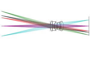
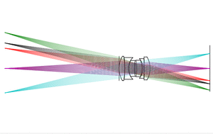 In the left picture, the aperture is defined by the first surface. In the right picture, the aperture is defined by a surface in the middle of the optical system.
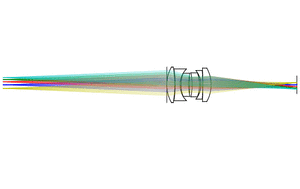
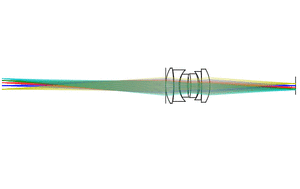 In the left picture, the system is telecentric (aperture at infinity) in the object space as the chief rays in the object space are all parallel. In the right picture, the system is telecentric in the image space as the chief rays in the image space are all parallel.
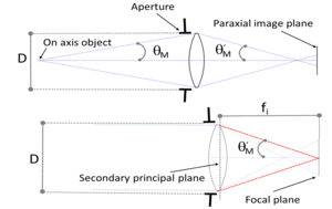 The aperture can be defined in several ways.
It can first be specified by the diameter D of the aperture itself.
It can also be defined by the half aperture angle θM in the object space. θM is the angle with the axis of a ray coming from the on-axis object and passing at the edge of the aperture in the object space (called marginal ray).
θM is often used to specify the aperture of illumination optics. For these systems, θM may be larger than 90°.
The aperture is commonly specified with the numerical aperture in the object space NA.
The aperture can be defined in several ways.
It can first be specified by the diameter D of the aperture itself.
It can also be defined by the half aperture angle θM in the object space. θM is the angle with the axis of a ray coming from the on-axis object and passing at the edge of the aperture in the object space (called marginal ray).
θM is often used to specify the aperture of illumination optics. For these systems, θM may be larger than 90°.
The aperture is commonly specified with the numerical aperture in the object space NA.
 where n is the refraction index in the object space.
The aperture is also often defined with the F number (common notation: F/N, F#, Fnumber). It is currently the case for many systems as for instance camera lenses.
where n is the refraction index in the object space.
The aperture is also often defined with the F number (common notation: F/N, F#, Fnumber). It is currently the case for many systems as for instance camera lenses.
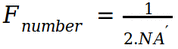 .
.
 . is the numerical aperture in the image space (n' is the refraction index in the image space). The larger the aperture, the larger the numerical aperture and the lower the F number.
For optical systems with small aperture and working for objects located at infinity, the F number is approximately the ratio of the focal length fi to the diameter D of the stop surface :
. is the numerical aperture in the image space (n' is the refraction index in the image space). The larger the aperture, the larger the numerical aperture and the lower the F number.
For optical systems with small aperture and working for objects located at infinity, the F number is approximately the ratio of the focal length fi to the diameter D of the stop surface : 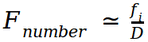 .
.
Geometric aberration formula
At this stage, it is necessary to give the definition of the expressions commonly used to describe aberrations.
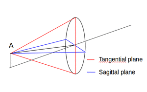 The tangential plane linked to the object A is the plane containing A and the optical axis of the system. Thus, it necessarily contains the aperture center (the aperture being supposed to be centered on the optical axis).
The sagittal plane linked to the object A is perpendicular to the tangential plane. It also contains A and the aperture center.
The tangential plane linked to the object A is the plane containing A and the optical axis of the system. Thus, it necessarily contains the aperture center (the aperture being supposed to be centered on the optical axis).
The sagittal plane linked to the object A is perpendicular to the tangential plane. It also contains A and the aperture center.
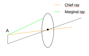 The chief ray linked to the object A is the ray coming from A and passing through the aperture center.
A marginal ray linked to the object A is a ray coming from A and passing at the edge of the aperture.
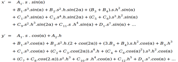
The coordinate x' and y' of the impact B in the observation plane of a ray coming from an objet A and propagating through an optical system can be calculated according to the formula below :.
The chief ray linked to the object A is the ray coming from A and passing through the aperture center.
A marginal ray linked to the object A is a ray coming from A and passing at the edge of the aperture.
The coordinate x' and y' of the impact B in the observation plane of a ray coming from an objet A and propagating through an optical system can be calculated according to the formula below :.
 .
.
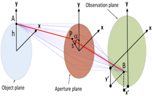 The object A is considered on the Y axis. h is its coordinate along the Y axis. P is the impact of the ray on the aperture in the object space. s and α are the cylindrical coordinate of P referred to the aperture (see the picture on the left).
This formula relates all the aberrations which are 5 in number : the spherical aberration, the coma, the astigmatism together with the field curvature and the distorsion.
This formula is a Taylor expansion. The first order terms (s.cos(α) and s.sin(α)) correspond to the terms of the gauss approximation. A2 coefficient is related to the magnification. A1 coefficient expresses a defocus and thus would be equal to "0" if the observation plane was the paraxial image plane. The higher order terms are related to the transversal geometric aberrations.
The third order terms are generally preponderant in optical system with a relatively small aperture. They are the "B" coefficients in the formula. They are also called Seidel coefficients.
B1 is related to the spherical aberration, B2 to the coma, B3 to the astigmatism, B4 to the field curvature and B5 to the distorsion. Note that this aberrations classification is exhaustive and therefore is also suitable for higher orders (5th order aberrations expressed through the "C" coefficients, 7th order aberrations not expressed in the above formula, etc.). For simplicity, the following sections are sometimes based on third order aberrations interpretation which are existing in any case and preponderant for slightly opened systems.
The object A is considered on the Y axis. h is its coordinate along the Y axis. P is the impact of the ray on the aperture in the object space. s and α are the cylindrical coordinate of P referred to the aperture (see the picture on the left).
This formula relates all the aberrations which are 5 in number : the spherical aberration, the coma, the astigmatism together with the field curvature and the distorsion.
This formula is a Taylor expansion. The first order terms (s.cos(α) and s.sin(α)) correspond to the terms of the gauss approximation. A2 coefficient is related to the magnification. A1 coefficient expresses a defocus and thus would be equal to "0" if the observation plane was the paraxial image plane. The higher order terms are related to the transversal geometric aberrations.
The third order terms are generally preponderant in optical system with a relatively small aperture. They are the "B" coefficients in the formula. They are also called Seidel coefficients.
B1 is related to the spherical aberration, B2 to the coma, B3 to the astigmatism, B4 to the field curvature and B5 to the distorsion. Note that this aberrations classification is exhaustive and therefore is also suitable for higher orders (5th order aberrations expressed through the "C" coefficients, 7th order aberrations not expressed in the above formula, etc.). For simplicity, the following sections are sometimes based on third order aberrations interpretation which are existing in any case and preponderant for slightly opened systems.
Spherical aberration
Let consider an optical system with spherical aberration (coefficients B1 for the third order spherical aberration, C1 for the fifth order spherical aberration,...) Rays from an on-axis object and making the same angle θ with the optical axis are focusing at the same point (image) because of the cylindrical symetry of the system. This appears in the Taylor expansion by the fact that the spherical aberration terms are not depending on α (see section related to the "geometric aberrations"). However, the position of this image depends on θ (or s in the Taylor expansion). At the limit angle θ = 0, the image coincides with the paraxial image. The spherical aberration represent the variation of image position depending on θ. The maximum distance between the image and the paraxial image is the longitudinal spherical aberration. The transverse spherical aberration is equal to the aberration spot diameter in the paraxial image plane. Note that the spot is circular because of the cylindrical symetry of the system. The spherical aberration depends on the position of the object plane, on the lens shape and obviously on the aperture size. It does not depend on the aperture position and on the distance of the object to the optical axis as the related coefficients in the Taylor expansion are proportionnal to s2.n+1. It means that the spherical aberration is the same everywhere in a given object plane.
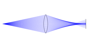
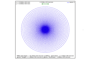 The two figures on the left show the ray tracing of a single spherical lens with spherical aberration (leftmost picture) and the associated spot diagram in the paraxial image plane (rightmost picture).
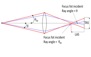 The left side scheme illustrates the case of a converging spherical lens. The larger the angle θ, the more the image moves away backwards from the paraxial image. The longitunal spherical aberration noted LAS on the picture is then negative, which means that the lens is undercorrected. In this particular case, the transverse spherical aberration is
  . The longitunal spherical aberration is positive for a diverging lens which is then overcorrected.
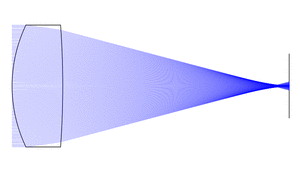
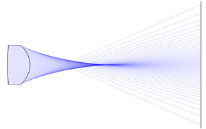 It is possible to minimize the spherical aberration of a single lens in certain conditions. That is for instance the case with an object at infinity and when the radius of curvature of the first facet is around 6 time smaller than the radius of curvature of the second facet (see left figure on the left side). Note that if the lens is reversed (right figure), the spherical aberration is no more minimized. Note also that the lenses displayed on the two picture seems different just because the pictures have different ratio vertical scale/horizontal scale. In general, when considering a lens with convex facets, the configuration with less spherical aberration is the following one : the facet with the smallest radius is oriented towards the "more parallel" rays.
In the general case, an optical system with spherical aberration can be either undercorrected or overcorrected. LAS is not necessary the distance d from the paraxial image to the marginal rays image : in many cases, LAS > d and it is the distance from the paraxial image to the image corresponding to an intermedate angle  .
The spherical aberration depends on the position of the object plane and on the aperture size. It does not depend on the aperture position and on the distance of the object to the optical axis as the related terms in the Taylor expansion are proportionnal to s2.n+1. It means that the spherical aberration is the same everywhere in a given object plane.
Most components as spherical lenses, spherical mirrors, plates with flat and parallel faces,...have spherical aberration whatever the object position. Some others like ellipsoidal or parabolic mirrors and dioptres have in general spherical aberration but may be rigorously stigmatic for particular object positions (see rigorous stigmatism tutorial).
An optical system can be corrected for the spherical aberration (generally partially up to a certain order) by using aberrated components that combined together finally minimize or cancel its effects. Also, a certain type of lenses with aspherial shapes can almost be totally corrected for spherical aberration, even for large apertures. These kind of lenses are for instance used for on-axis objects, for example to inject the beam from a VCSEL (Vertical Cavity Surface Emitting Laser) which emitting area is small (in the range of the micron2) into a single mode fiber optic. A group of two lenses, the first one collimating the beam and the second one focusing the beam at the fiber entrance can be used for an optimal coupling. There are other solutions for minimizing spherical aberration like using a Schmidt plate before a spherical mirror when the object is at infinity...
.
The spherical aberration depends on the position of the object plane and on the aperture size. It does not depend on the aperture position and on the distance of the object to the optical axis as the related terms in the Taylor expansion are proportionnal to s2.n+1. It means that the spherical aberration is the same everywhere in a given object plane.
Most components as spherical lenses, spherical mirrors, plates with flat and parallel faces,...have spherical aberration whatever the object position. Some others like ellipsoidal or parabolic mirrors and dioptres have in general spherical aberration but may be rigorously stigmatic for particular object positions (see rigorous stigmatism tutorial).
An optical system can be corrected for the spherical aberration (generally partially up to a certain order) by using aberrated components that combined together finally minimize or cancel its effects. Also, a certain type of lenses with aspherial shapes can almost be totally corrected for spherical aberration, even for large apertures. These kind of lenses are for instance used for on-axis objects, for example to inject the beam from a VCSEL (Vertical Cavity Surface Emitting Laser) which emitting area is small (in the range of the micron2) into a single mode fiber optic. A group of two lenses, the first one collimating the beam and the second one focusing the beam at the fiber entrance can be used for an optimal coupling. There are other solutions for minimizing spherical aberration like using a Schmidt plate before a spherical mirror when the object is at infinity...
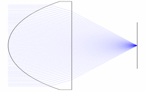
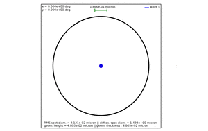 The leftmost picture shows the ray tracing of a lens which is flat on one side and aspherical on the other side. The aspherical side is optimized to correct almost perfectly the spherical aberration for an object at infinity. Its spot diagram (right picture) shows a spot much smaller than the Airy disk (black circle) defining the diffraction limit of the system (see the "diffraction" tutorial).