Handy Calculations
Overview
The Handy Calculations tool provides a comprehensive set of specialized calculation pages dedicated to various fields in photonics. Currently, 287 pages are available, covering areas such as diffraction, fiber optics, geometrical optics, interference, lasers, optoelectronics, polarization, and radiometry/photometry.
A dedicated unit conversion section is also available. Each calculation page includes contextual help via tooltips to enhance clarity and usability.
Find a Calculation Using the Menus
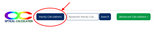
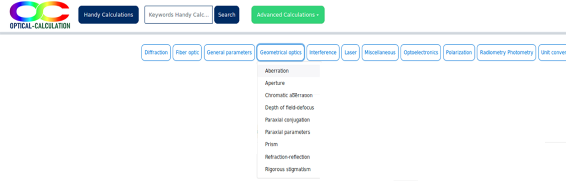
You can access calculation pages using the two-level dropdown menu that appears when you click on the "Handy Calculations" link at the top-left corner of each page. These dropdowns correspond to various photonics fields, and their submenus link to specific topics.
By default, the first calculation page related to the selected topic is displayed. If that’s not the one you need, browse the "list of links" in the left-hand panel to find a more relevant page. If none of them suits your needs, feel free to contact us — we will do our best to assist.
Find a Calculation Using the Search Bar
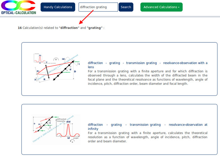 Alternatively, you can search for a specific calculation by entering keywords into the search bar located in the header. After clicking the Search button, a list of pages matching all the entered keywords will be displayed.
Each result includes a title, a short description, and sometimes a visual diagram. You can access a page directly by clicking on its title or, if available, on the diagram.
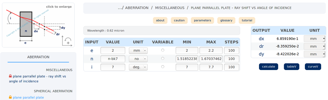
Calculation page overview
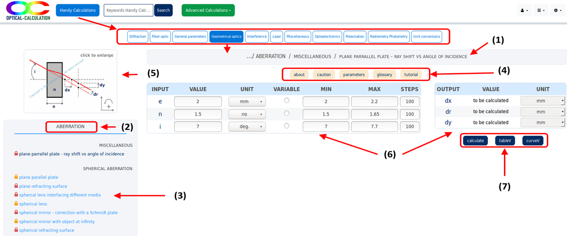
Each calculation page consists of several sections:
- a list of links (3) to related calculation pages based on the topic (2) (displayed on the left-hand side),
- one or two calculation tables (6) depending on the format used, with buttons (7) to process the calculation,
- links to tooltips and a tutorial (4) (located above the calculation tables),
- the navigation path (1) leading to the current page (displayed above the tooltips and tutorial link),
- an illustrative diagram (5) present on most pages, which can be enlarged by clicking on it (top-left of the page).
List of links
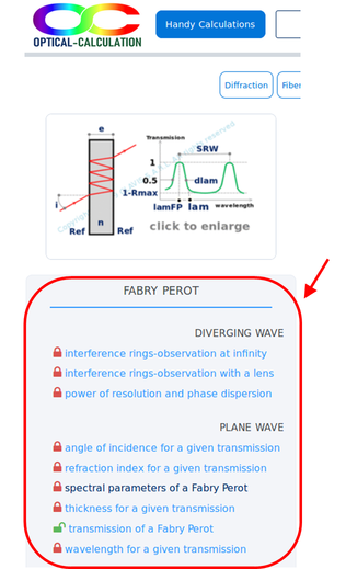 To enhance clarity, the list of calculation pages on the left may be organized by subtopics (displayed in grey small caps). Users can access a specific calculation by clicking on its title in the list. The selected title is highlighted with a darker color. A padlock icon appears to the left of each calculation title in one of the following ways:
- indicates that the calculation is freely accessible without logging in,
- means the calculation is accessible if the user is logged in and holds a Student or Premium license,
- means the calculation is only accessible with a Premium license.
More details about access levels and available features are provided on the features page.
Processing calculations
Each Handy Calculation page is designed to perform calculations based on input data entered by the user.
There are two calculation modes:
In the fixed mode, all input parameters are set, and the calculation is performed accordingly.
In the varying mode, one input parameter is varied while the others remain fixed. The varying mode is available on all pages except those for unit conversions, glass catalogs, and the wavelengths page.
Additionally, there are two layout formats used in calculation pages:
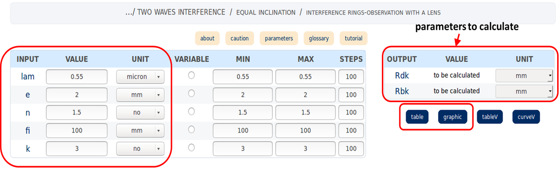
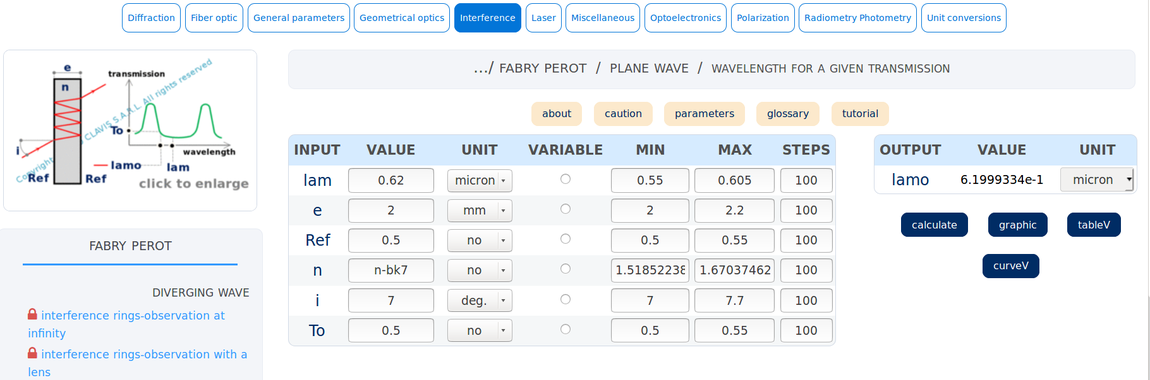
Pages using the two-table format include two tables: one for entering input parameters ("input" table) and another for displaying results ("output" table) in fixed mode.
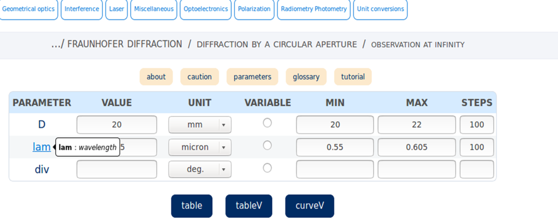
Pages using the single-table format include one table ("parameters" table) where both input and output are handled. The user selects the parameter to be calculated by leaving its value cell empty. All other cells must be filled with input values. This setup allows any parameter to be derived from the others.
Depending on the page, the number and label of buttons for performing calculations may vary.
In all cases, buttons labeled "tableV" and "curveV" are used for varying mode calculations. All other buttons are used for fixed mode calculations.
Descriptions of input and output parameters are available in tooltips when hovering over their labels.
Calculating in fixed mode
Input/output units can be selected in the "unit" column. The calculation is performed and results are displayed in the appropriate table after clicking the "calculate" or "table" button (one of them is always present on the page).
On some pages, results can also be displayed graphically by using the "graphic" or "curve" buttons, or any other custom button.
Two-table format
Single-table format
Input values can be entered in either numerical or scientific format, using up to 14 digits.
Output values are displayed in scientific notation with a minimum of 2 and a maximum of 6 decimal places.
Remember: in the single-table format, the "value" cell of the parameter to be calculated must be cleared; otherwise, an error message will be shown.
Calculating in varying mode
Except for the conversion pages, it is possible to perform a calculation by varying one input parameter across a range of values. This parameter is selected via its corresponding radio button in the "variable" column. You must enter its minimum value valmin and maximum value valmax in the "MIN" and "MAX" cells, respectively. The number of intermediate values minus one is defined in the "STEPS" cell. The calculation is performed for each value of the parameter:

i varies from 0 to "STEPS".
Input values can be entered in numerical or scientific format using up to 8 digits. Results are displayed in scientific notation. Input and output values are displayed using 6 and 4 decimal places, respectively.
The number of values ("STEPS" column) is generally limited to 200, but this limit may be reduced for time-consuming calculations.
As in fixed mode, in the single-table format, the "value" cell of the parameter to be calculated must be empty. Additionally, the variable parameter cannot be the one being calculated.
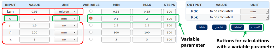
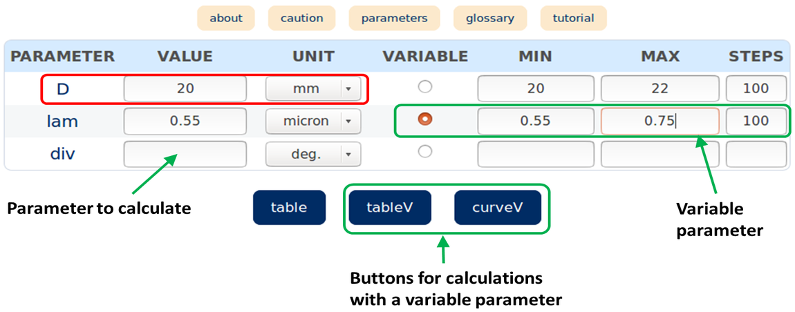
The results can be displayed either in a table or as curves.
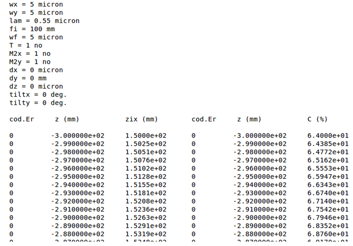
Results appear in a table after clicking the "tableV" button. For each output, three columns are shown:
- The first column labeled "cod.Er" displays an error code: 0 means the calculation was successful, 1 means it failed due to being impossible or not accurate enough.
- The second column shows the value of the varied input parameter.
- The third column contains the output value.
Fixed input values are displayed at the top of the table.
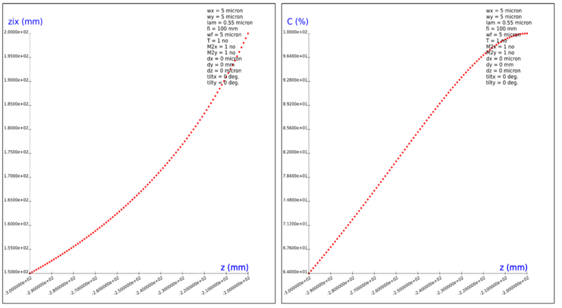
Results appear as curves after clicking the "curveV" button. There is one curve per output parameter. For each curve:
- The horizontal axis (abscissa) represents the values of the varied parameter.
- The vertical axis (ordinate) represents the calculated output values.
Fixed input values are displayed at the top of the graph.
Caution
By default, input fields are pre-filled to allow immediate calculation. These default values are automatically loaded. In some cases, they may cause errors because they are shared across multiple pages and may not be relevant for specific calculations.
Users can replace them with their own values, which might also lead to errors depending on the context. While assigning unique default values per page could avoid this, using common values can be helpful when chaining calculations across multiple pages without re-entering data.
In some cases, the message "not possible" may appear directly in the result cell without a prior error alert. This occurs when intermediate tests during calculation prevent the display of realistic or precise values. Unlike pre-checks (e.g., avoiding division by zero), these tests cannot trigger a full error message and are instead shown directly in the cell.
Using very small or very large values can lead to significant rounding errors. When such rounding is detected, the result may be displayed as a very small or very large number. For instance, angles may be rounded to the order of 10-6 radians, while large distances might be rounded to 10+12 mm.
In single-table pages where any parameter can be computed from the others, discrepancies may occur when re-computing an input value from prior results due to display precision limits. These differences are usually minor but can sometimes be significant — e.g., when recalculating "dark current" in the "shot noise current" page under certain extreme conditions. Higher display precision would fix this but would also cause issues in current display formats.
When a calculation involves a varying parameter, its values range from a minimum to a maximum defined in the "MIN" and "MAX" fields. These are usually pre-filled — except for the default output parameter in single-table format, where users must manually define them.
Make sure that the maximum value is strictly greater than the minimum. If the default value of a parameter is zero, its min and max are also initially set to zero and must be changed accordingly.
Lastly, note that integer-type parameters (e.g., diffraction orders) cannot be used as variable parameters.
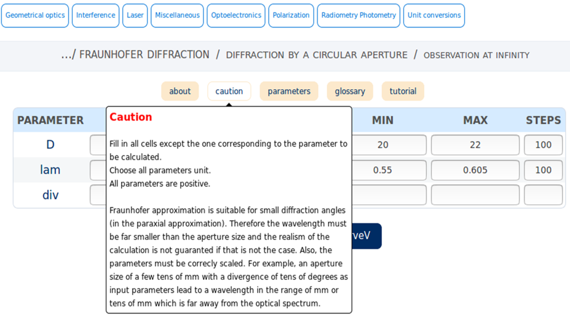
tooltips
Links to tooltips ("about", "caution", "parameters", "glossary") are provided to help you better understand the calculations. They can be accessed from the menu above the calculation table(s). Here’s what each tooltip does:
- "about" explains what the calculation does.
- "caution" outlines key considerations when entering input data.
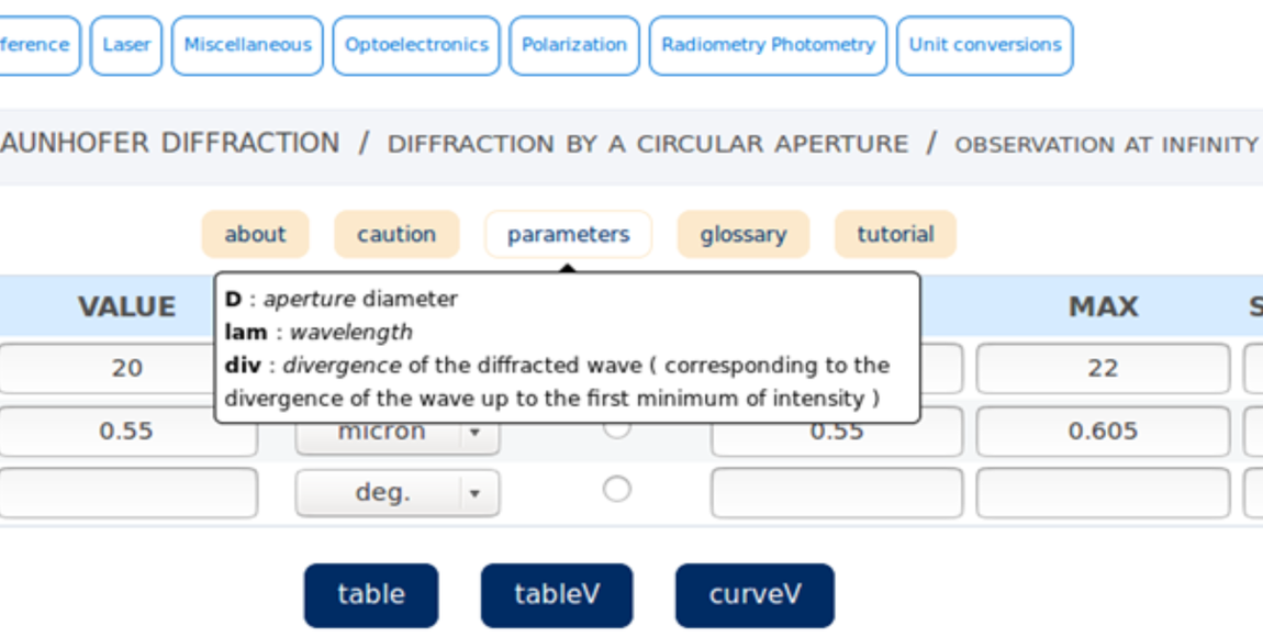
- "parameters" describes the meaning of each parameter used in the calculation.
- "glossary" defines technical terms used on the page or related to the calculation.
A link to a tutorial related to the calculation topic is also displayed to the right of the tooltips menu.
Tooltips appear when you hover your mouse over the corresponding label. You can also display their content in a separate page by clicking on the label.
In addition to the "parameters" tooltip, each parameter’s definition also appears in a pop-up when you hover over its label in the "input", "output", or "parameters" column.
Here is an example of a tooltip displayed when hovering over the "caution" link:
Here is an example of a tooltip displayed when hovering over the "parameters" link:
Here is an example of a pop-up displayed when hovering over a parameter label:
Using the glass catalog and choosing wavelengths
In some calculation pages, the refractive index is an input parameter. You can enter either a numerical value or a glass reference.
Catalog page
You may either input a value directly or select a glass reference from the catalog (path: "handy calculations/General parameters/catalogs").
On the left side of this page, multiple catalog links are available. Once you select a catalog, you can choose a glass reference in the "glass" cell and calculate the refractive index for the wavelength entered in the "lam" cell. The Abbe number and minimum wavelength for acceptable transmission are also displayed.
These values help guide the selection of a suitable reference for the intended calculation.
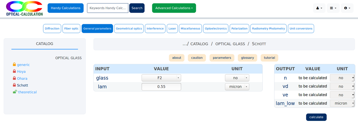
Note: Only the "theoretical" glass can be used without logging in.
The "generic" catalog is available with a Student license.
All other catalogs require a Premium license.
Entering a glass reference as a refractive index
On some pages where both the refractive index and wavelength are inputs, if you enter a glass reference instead of a value in the refractive index cell, the system will use the index of that glass at the specified wavelength.
On other pages where the wavelength is not an input, entering a glass reference in the refractive index field will cause the system to use the default wavelength (displayed at the top of the input tables during calculation).
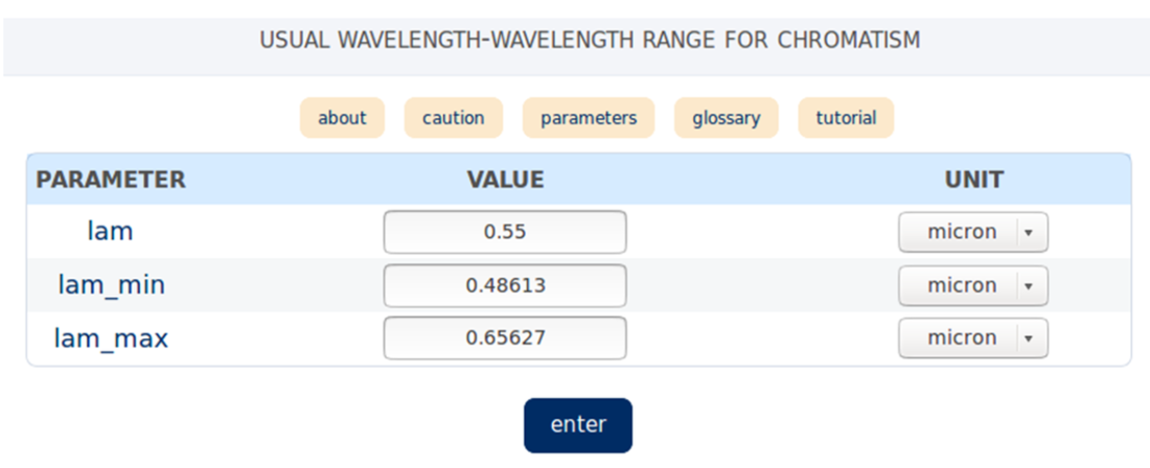
Initially, the default wavelength is 0.55 microns. You can change it by going to the wavelength page and entering a new value in the "lam" cell.
If the current page uses wavelength as an input, the entered value is saved as the new default for future calculations.
On that same page, you can also modify the "lam_min" and "lam_max" values, which define the range used for chromatism-related calculations.
Note: It is required that lam_min < lam < lam_max; otherwise, an error message will be shown.
For chromatism calculations, instead of manually entering the refractive indices for the minimum and maximum wavelengths of the spectrum, you can enter a glass reference. The corresponding refractive indices will then be automatically retrieved for those wavelengths.
By default, the minimum and maximum wavelengths are 0.48613 µm and 0.65627 µm, respectively, but you can modify them. These values are displayed at the top of the input table once the calculation is performed.
When the Abbe number (constringence) is an input, it can be entered either numerically or via a glass reference. In the latter case, the value associated with the selected glass is used in the calculation.
Optical software
Introduction
The Optical software is a versatile tool that allows for more complex computations than the Handy Calculations pages. It focuses on the analysis and optimization of optical systems and simulates real ray propagation. In addition, paraxial and radiometric calculations are available, as well as modeling for laser beam propagation and fiber coupling.
Almost any type of system can be simulated — up to 22 surfaces can be defined. Various surface types are supported: spherical, conical, aspherical, toroidal, biconical, paraxial, and paraxial without rotational symmetry. Gratings are also supported in both transmission and reflection. Surfaces can be tilted and decentered. Moreover, components from catalogs can be imported directly for simulation.
The aperture can be defined using different criteria: numerical aperture, half-angle, surface diameter, and f-number. Its position is defined by a specific surface within the system. Alternatively, the system can be telecentric in either the object or image space. Circular and rectangular apertures/obscurations are supported and can be decentered.
Up to 7 different wavelengths and 7 different fields can be defined.
Radiometric calculations can be performed using various source types (including blackbodies and grey bodies) with different shapes: point, circular, rectangular, cylindrical, and annular.
Numerous options are available for both calculations and results display. Input data can be saved locally on the user's computer (note: no data is stored on the "optical-calculation.com" server).
A wide range of analysis and optimization features are available.
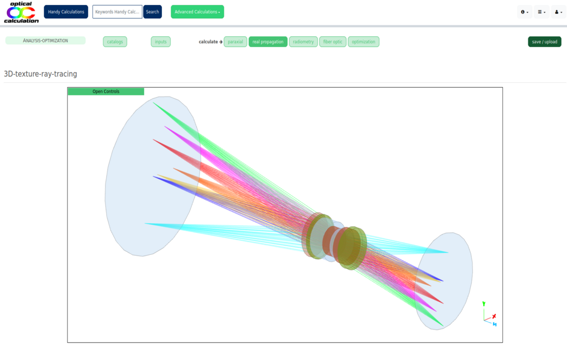
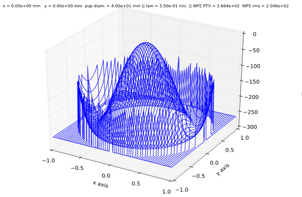
Among other capabilities, the software can perform 3D texture ray tracing, spot diagrams, ray aberration analysis, wavefront error evaluation, point spread function (PSF), and modulation transfer function (MTF) analysis. It can also evaluate the optimal position of the observation surface based on spot size.
Additional features include paraxial and chromatic aberration analysis, as well as evaluation of the power transmitted from a light source. Laser beam propagation and coupling efficiency into single-mode or multimode fibers are also supported.
Lastly, numerous surface parameters and merit function criteria can be used for optimization.
Overview
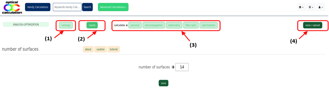
The "Optical software" can be accessed by clicking the "Access" button in the website’s main menu, then selecting the "Optical software / Analysis-optimization" link.
On the landing page, the menu for input data processing is located in the left column (1), while the calculation menu is in the top row below the banner (2).
The landing page is used to save the optical system data currently loaded into the software or to upload a system from a file. This page can also be accessed from anywhere in the software by clicking the "save/upload" button in the left menu. Further details on saving and uploading are provided in the relevant section. Note that a biconvex lens is loaded by default.
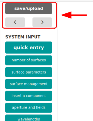
Input processing (1)
Input data is handled via buttons located in the left column menu.
- The "save/upload" button lets you save the currently loaded system or upload one from a file.
- The "<" button returns to the previously loaded system, while the ">" button cancels the previous action.
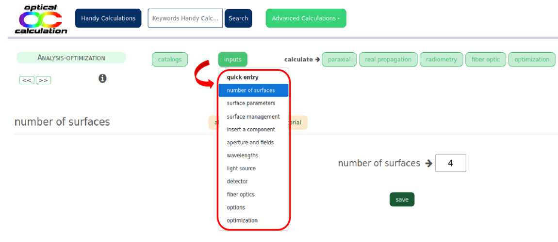
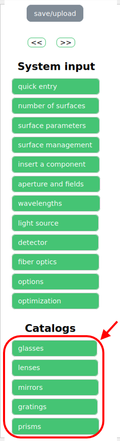
- The "System input" menu defines all system input parameters.
- The "Catalogs" menu allows filtering of components from the catalogs.
The "System input" menu includes buttons that lead to pages for entering parameters:
- "quick entry" (for directly defining a system using catalog components),
- "number of surfaces" (to set how many surfaces the system has),
- "surfaces parameters" (to enter parameters for each surface),
- "manage surfaces" (to add, remove, or flip surfaces),
- "insert a component" (to insert or replace a system with a catalog component),
- "aperture and fields" (to define aperture and field positions),
- "wavelengths" (to define the wavelengths used),
- "light source" (to define radiometric or laser parameters),
- "detector" (to define detector parameters for MTF analysis),
- "fiber optic" (for fiber coupling calculations),
- "options" (to define additional parameters for calculations or display),
- "optimization" (to define optimization parameters).
The "Catalogs" menu includes several buttons ("glasses", "lenses", "mirrors", "gratings", "prisms", "windows") linking to selection pages with filter options based on user-defined criteria.
Calculation processing (2)
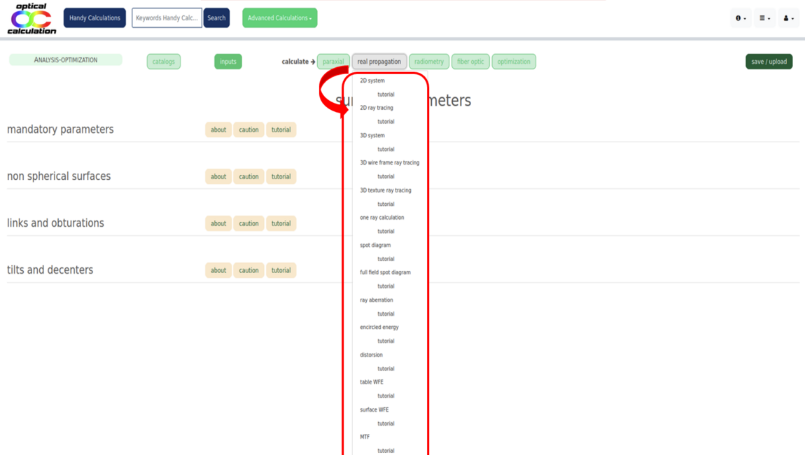
Below the banner, the "Calculate" menu displays several dropdowns for analyzing or optimizing the optical system. Each dropdown ("paraxial", "real propagation", "radiometry", "fiber optic" and "optimization") contains links to calculations and their associated tutorials.
The "paraxial" menu includes:
- "conjugation" (paraxial image and system parameters),
- "longitudinal chromatism" (image position vs. wavelength),
- "aperture" (paraxial aperture in object/image space),
- "laser beam propagation" (paraxial laser beam analysis).
The "real propagation" menu includes:
- "2D system", "2D ray tracing", "3D system", "3D wireframe ray tracing",
- "3D texture ray tracing", "single ray propagation",
- "spot diagram", "full field spot diagram", "ray aberration",
- "encircled energy", "distortion", "table WFE", "surface WFE",
- "MTF", "full MTF", "best focus", "PSF", "PSF cut-out",
- "relative laser beam intensity",
- "vignetting", "SAG".
The "radiometry" menu includes:
- "transmitted flux" (calculates transmitted power from a light source).
The "fiber optic" menu includes:
- "laser coupling in a single mode fiber optic",
- "laser coupling in a multimode fiber optic".
The "optimization" menu includes:
- "DLS cycles" (Damped Least Squares optimization),
- "DLS-cycles-random" (same, from randomly selected starting points).
"System input" pages
Each link in the "System input" menu leads to a page containing the following elements:
- One or more tables for entering parameters,
- Contextual support via the beige buttons ("About", "Caution", and "Tutorial") located at the top of each table for better understanding and usability.
Input tables
The input tables vary from page to page. They may include different types of input fields: text fields, checkboxes, dropdown menus, and radio buttons.
Parameters are only saved after clicking the corresponding "Apply" button. If multiple tables are present, you must click "Apply" for one table before entering data into another. Do not input data into multiple tables and click all "Apply" buttons afterward — this could result in incorrect behavior.
The maximum number of characters allowed depends on the parameter type, with a general limit of 14 characters. Consequently, the maximum number of decimals is also limited — up to 13 for positive numbers and 12 for negative ones in standard notation.
Scientific notation can be used to bypass these limits (e.g., you may enter 1.23e-12 instead of 0.00000000000123).
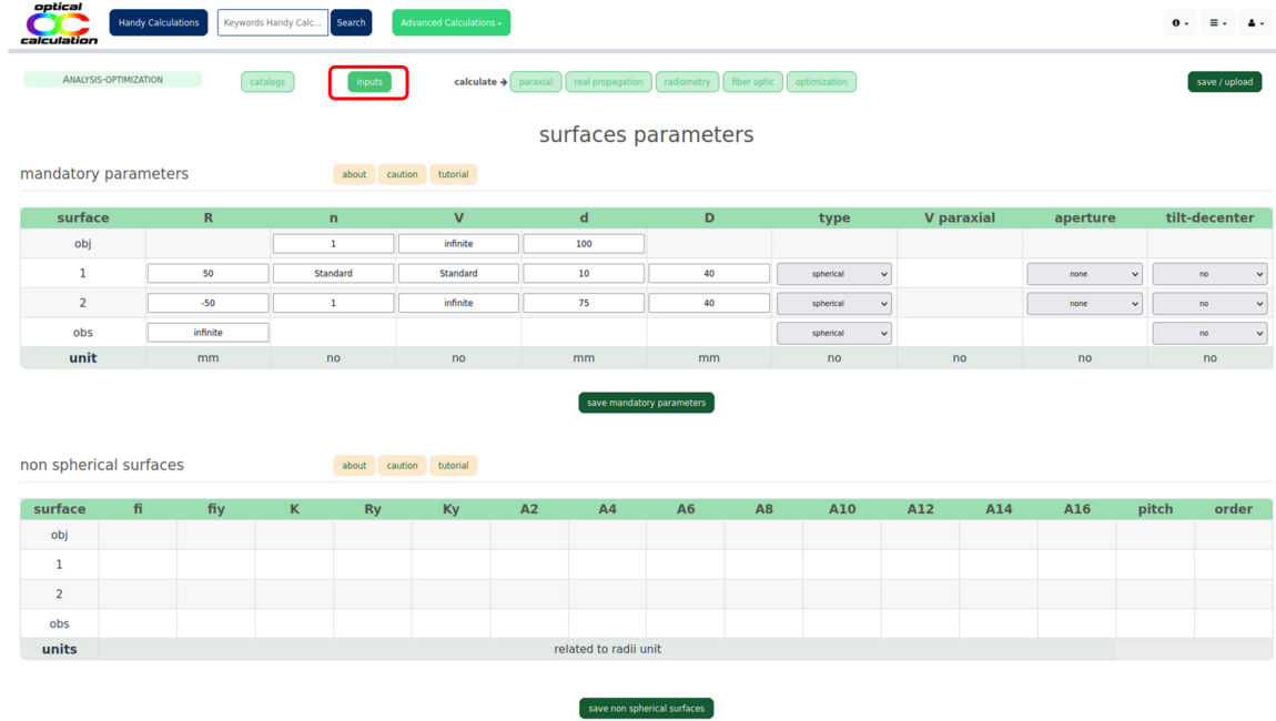
Exception: "Surfaces parameters" page
If possible, 2D and 3D views of the optical system are displayed at the top of the page. Below this, buttons labeled "Sx" (where "x" is the surface number) are shown. Unlike other pages, this one does not display all tables by default.
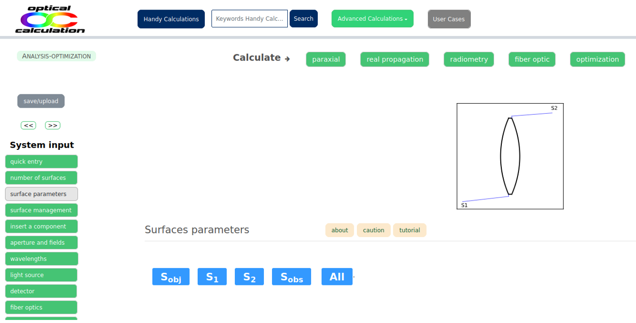
Clicking on a button displays the table for the corresponding surface. Clicking the same button again hides the table. This allows you to show only the desired tables.
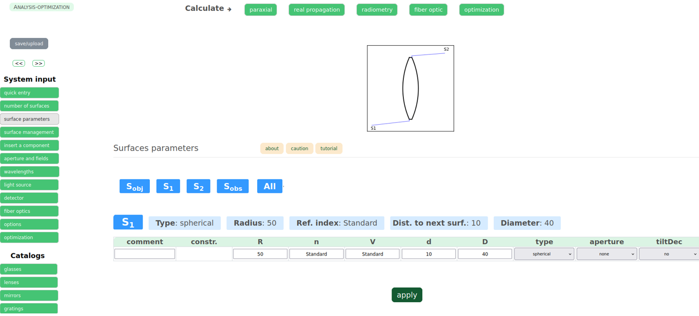
The "All" button displays all surface tables at once and hides them again if clicked a second time.
Each surface has a table with at least one row of mandatory parameters (e.g., radius of curvature, refractive index and constringence of the next medium, distance to the next surface). Other rows are revealed by selecting surface types, aperture types, tilts, and decentering options.
It's also possible to constrain one surface relative to another. In that case, an additional row is displayed to define the relationship between the surfaces.
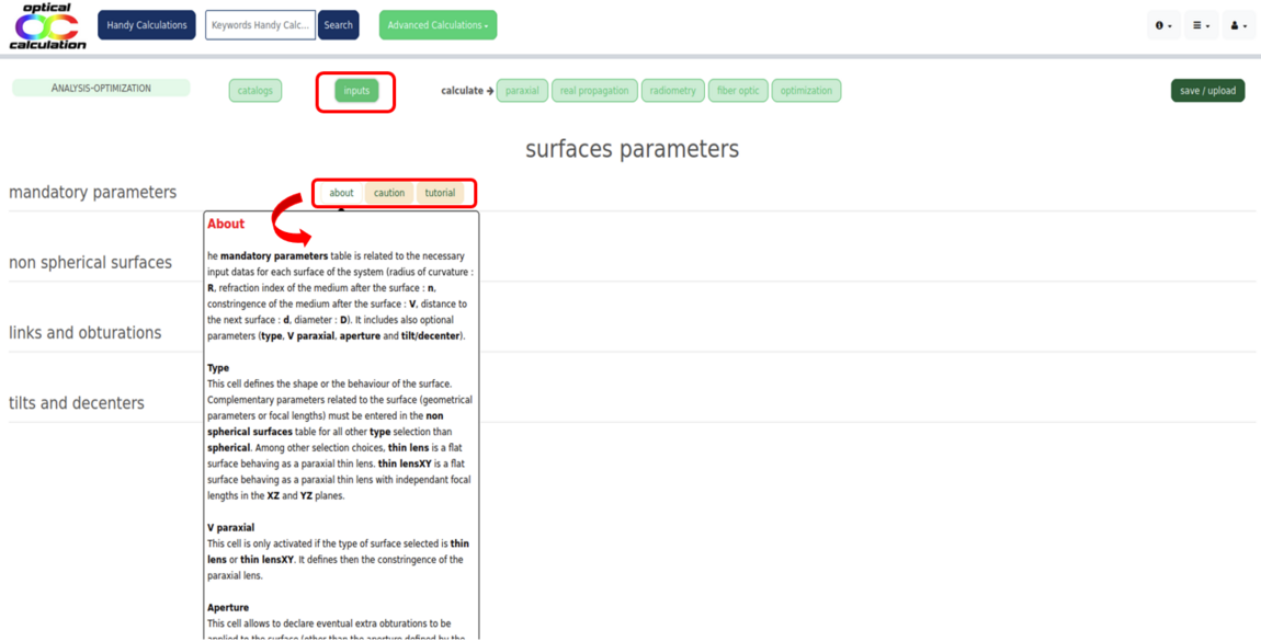
Contextual support
Like in the "catalogs" pages, each input table includes contextual support. When hovering over the beige "About" and "Caution" buttons at the top of the table, tooltips appear with additional information.
These can also be displayed in a separate page by clicking the buttons.
- "About" explains the different parameters in the table.
- "Caution" gives guidance on how to properly enter the parameters.
- The "Tutorial" link opens a detailed guide about the relevant input page.
Order of input parameters
A default system (usually a lens) is loaded automatically. If your system is different, you should define the parameters in the following order:
1) Number of surfaces (via "number of surfaces"),
2) Mandatory surface parameters (via the "mandatory parameters" table in "surfaces parameters"),
3) Aperture (via the "aperture" table in "aperture and fields").
This order helps avoid inconsistencies. Errors or conflicts are detected as you enter data. All other parameters can be entered in any order.
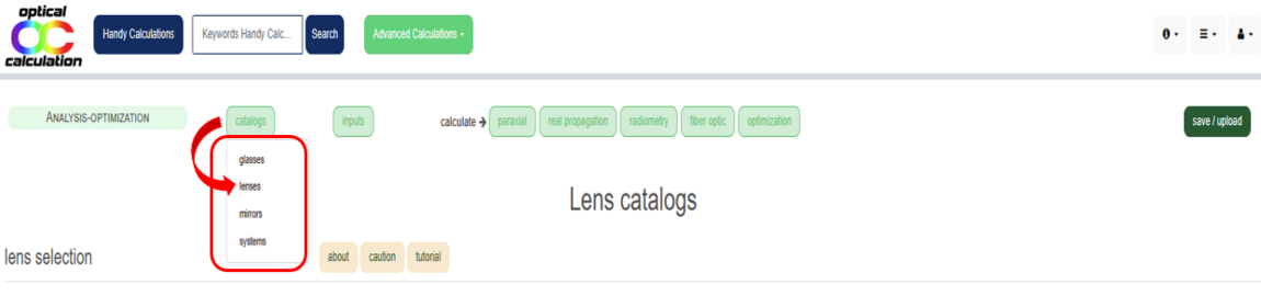
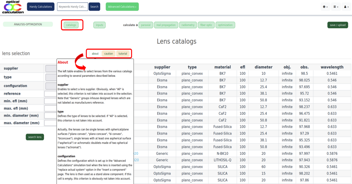
"Catalogs" pages
Catalogs are accessible via the "catalogs" dropdown menu, which offers access to five different catalogs: "glasses", "lenses", "mirrors", "gratings", "prisms" and "windows.
Catalog tables
Regardless of the selected element type ("glasses", "lenses", "mirrors", "gratings", "prisms" or "window), a selection table appears on the left side of the page. This table allows you to filter components using various criteria.
Once the selection table is validated, the matching elements are displayed in a result table on the right, along with their main characteristics.
Note that simplified catalogs are available to all visitors for browsing. Logged-in users with a "Premium license" gain access to complete catalogs for simulation purposes, while those with a "Student license" only have access to reduced versions (see the "features" page on the website).
Contextual support
Each "catalog" page includes contextual assistance. Tooltips with information related to the specific catalog appear when you hover over the beige "About" and "Caution" buttons at the top.
These tooltips can also be opened in a separate page by clicking on the respective buttons.
- "About" explains the different parameters found in the selection and result tables.
- "Caution" provides recommendations for correctly entering filter criteria in the selection table.
- The "tutorial" link opens a detailed guide on the chosen catalog and offers practical tips for component selection.
"Save / upload" button
You can save or upload input parameters used in "Optical software" via the "save/upload" button at the top of the "System input" menu.
Below this button, two additional buttons allow you to load the previously saved setup or move forward to the next one.
Clicking this button opens a new page with three sections:
(1) A section on the left with a "save" button,
(2) A section on the right for uploading an OC file,
(3) A section below for uploading a Zemax file.
This page is also the default landing page of the software.
The quickest way to save your input parameters is to click the "save" button directly. The parameters are then downloaded to your computer’s "Downloads" folder as a file named optical-calculation_"userLogin".oc, where "userLogin" is a simplified version of your email (dots and @ removed).
You can also enter a custom filename in the designated field before clicking "save".
Input data can be uploaded from a previously saved file or from your "optical-calculation.com" library. To do this, select the file using the "Browse..." button in the "Upload Optical-Calculation file" section, then click "upload OC file". After uploading, you can verify success by checking the updated input tables.
⚠️ For maximum privacy, files are never stored on the "optical-calculation.com" server.
You can also upload a .zmx file (Zemax format) by selecting it via the "Browse..." button and clicking "upload Zemax file" in the "Upload ZEMAX file (centered system)" section. This feature currently does not support coordinate breaks, so it is intended for centered systems only.
If your file fails to upload, please contact us — this is often due to a glass reference mismatch between your Zemax file and our database, or a reference missing from our catalogs. In both cases, we can adjust our database accordingly.
Important: To avoid losing your data, we strongly recommend saving your input parameters regularly. These data are lost once your session expires.
Output pages
A calculation is executed by clicking the corresponding button in the "Calculate" dropdown menu. Depending on the type of calculation selected, the result is displayed as a graph, a table, or plain text.
A tutorial is available for each calculation via the "tutorial" link located just below the corresponding button. The tutorial explains how the calculation is performed and provides information about optional settings that can be used to customize the process.
Other features
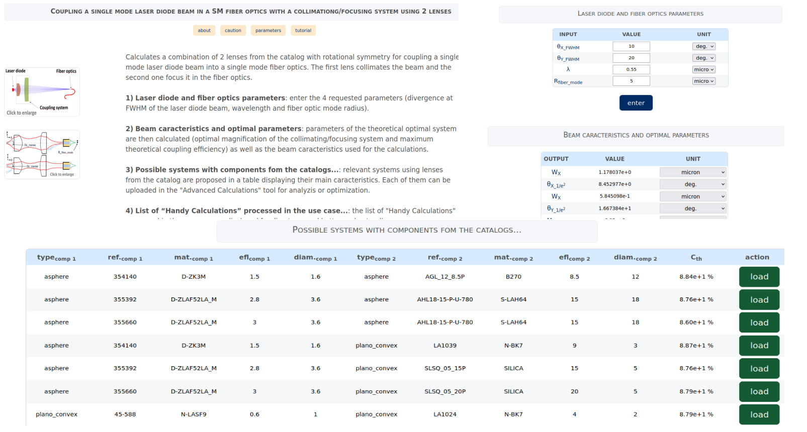
Solvers
 Clicking the 'Solvers' button opens a page displaying a list of available solvers. Selecting an item from the list automatically loads the corresponding solver interface.
Please note that the list of user cases will be extended over time based on user requests.
Each solver addresses a complete user case by automating the required sequence of calculations and optimizations. In most cases, multiple solutions are provided with a single click, and can be directly uploaded into the "Optical Software" for further analysis. The associated "Handy Calculations" used in the preliminary steps are also displayed.
Each user case page includes contextual information accessible through the beige buttons ("about", "caution", "parameters", and "tutorial").
Tutorials

A list of links to tutorials is accessible via the "tutorial" item in the general drop-down menu (on the right side of the header). Each link opens a diagram associated with the corresponding tutorial. The topics covered in the tutorials are the same as those addressed in the "Handy Calculations" section.
Each calculation page also includes a link to a specific tutorial page, as mentioned earlier.
Please note that these tutorials are only available to logged-in users.
Glossary
The Glossary is accessible via the "Glossary" link in the general drop-down menu at the top right of the header. It provides definitions for many terms commonly used in photonics.