
paraxial conjugation
Optical system
Optical systems are assemblies of optical components for redirecting the light in a controlled manner. Some of them are used for illumination like for instance reflectors and lenses in car headlights. Some of them can be used to shape a laser beam for example before its injection into a fiber optic. Optical systems are also used in experimental set up to bring light into a photodetector. Many of them are used to create the image of an object in order to bring it closer to the observer, magnify it, project it on a screen, etc. Among the imaging systems, the most common presently are the camera lenses enabling to conjugate a scene on the sensitive area of the camera. In imaging systems, the objective is to focus at one point all rays coming from a punctual object and therefore create the sharpest image of a scene.
Gauss conditions
Gauss conditions apply to all optical systems with a symmetry of revolution around an axis called the optical axis. Indeed, unlike some particular cases described in the "rigorous stigmatism" tutorial, most optical systems have aberrations. This
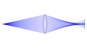
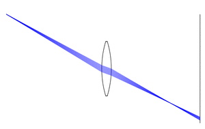
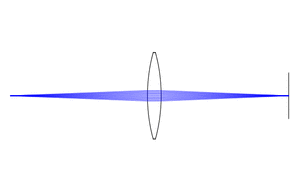
means that rays coming from a punctual object are not converging rigorously to an image point after passing through the optical system. This phenomenom is amplified when the angle of the rays with the optical axis and/or the object distance to the optical axis increase. The smaller these angles and distance, the more the rays converge towards a point. Thus, for sufficiently small rays angles (the optical system is then said to have a small aperture - see "aberrations" tutorial) and object distance, the system can be considered as stigmatic. It is then said that the optical system works in Gauss conditions or paraxial conditions. This approached stigmatism is also called paraxial conjugation. It is illustrated in the three pictures below. They all show a ray tracing with the same lens but with different object and/or aperture. The left picture illustrates the case of an on-axis object and a significantly large aperture preventing from approached stigmatism. In the middle one, the aperture is rather small but the object is too far from the axis to allow approached stigmatism. In the right one, the object is on axis and the aperture is the same than in the middle picture : the approached stigmatism is reached.
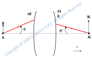 For rigorous stigmatism, Abbe sinus relation applies (see tutorial "rigorous stigmatism). In Gauss conditions and thus for approached stigmatism, this relation applies only for small ray angles and can be approximlated as follows :
 .
.
A and Ai are conjugated by the optical system, B and Bi are such that A to B and Ai to Bi vectors are perpendicular to the optical axis. AB and AiBi are the algebric distances respectively from A to B and from Ai to Bi. n0 and n1 are the refraction indexes respectively in the object and in the image space.
θ and θ' are the angles with the optical axis respectively of an incident ray obviously passing through A and of its emerging ray passing through Ai. As θ and θ' are small,  .
.
Characteristic parameters of the optical system under Gauss conditions can be calculated. Whatever a punctual object, they enable to define the position of what is called its paraxial image or its conjugated through the optical system. These parameters are the paraxial parameters. They are detailed in the "paraxial parameters" tutorial. Their knowledge is necessary to understand the rest of the tutorial.
Transverse magnification
For optical systems working in Gauss conditions, the paraxial image Pi of a plane P perpendicular to the optical axis
is also a plane perpendicular to the optical axis.
 Accordingly, for a segment joining two points A and B in the plane P,
the conjugated segment AiBi is contained in Pi and is perpendicular to the optical axis.
The transverse magnification m ( currently called "magnification" ) is the ratio AiBi/AB where AB and
AiBi are the algebric lengths of the considered segments. Consequently, m is an algebric value.
Accordingly, for a segment joining two points A and B in the plane P,
the conjugated segment AiBi is contained in Pi and is perpendicular to the optical axis.
The transverse magnification m ( currently called "magnification" ) is the ratio AiBi/AB where AB and
AiBi are the algebric lengths of the considered segments. Consequently, m is an algebric value.
m is constant whatever the points A and B in the plane P.
It is negative when AB and
AiBi have opposite signs (which means that object and image are oriented in opposite directions). It is positive when AB and
AiBi have the same sign ( which means that object and image are oriented in the same direction ).
m depends on the paraxial parameters of the optical system ( focal lengths, principal planes location ) and P position.
Conjugation formulas
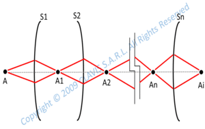 An optical system is in general made of several reflecting or refracting surfaces. The paraxial image of an object can be determined with a step by step process by calculating first the intermediate paraxial image of the object by the first surface, then calculating the conjugate of this intermediate image by the second surface and so on. This process is tedious. However, it is used for calculating the paraxial parameters detailed in the "paraxial parameters" tutorial as the principal planes, focal planes and focal lengths. Once these parameters determined, they are used in simple formulas to define the conjugation between an object and its paraxial image through the optical system.
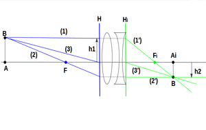 The position of the paraxial image through an optical system can be obtained geometrically considering two characteristic rays (ray (1) and ray (2)) coming from an off-axis object. The first ray (1) is parallel to the optical axis and the second one (2) goes through the front focal point. Both rays (1) and (2) intercept the primary principal plane at the respective heights h1 and h2 (h1 and h2 being respectively the object height and the image height). Therefore, emerging rays (1') and (2') respectively from rays (1) and (2) intercept the secondary principal plane at the same height than their incident ray on the primary principal plane. ray (1') focuses on the back focal point while ray (2') is parallel to the optical axis. The paraxial image of the object is the intersection of ray (1') and ray (2'). The plane passing through this point and perpendicular to the optical axis is the conjugated by the optical system of the plane perpendicular to the optical axis and passing through the object.
When the refraction indexes of the object and image spaces are the same, one can consider a third ray (3) coming from the object and intercepting the object nodal point (also front or primary nodal point). After passing through the optical system, the third ray (3') passes through the image nodal point (also back or secondary nodal point) and its direction is unchanged. Obviously, this third ray (3'), ray (1') and ray (2') are intersecting at the same point (corresponding to the paraxial image) of the object. In the general case where refraction indexes before and after the optical system are not the same, the direction (3') is not parallel to the direction (3).
According to the paragraph above, the position of the paraxial image plane is given by the position of its intersection Ai with the optical axis. A is the intersection of the object plane with the optical axis.
si is the algebric distance from the secondary nodal point Ni to Ai and can be calculated from the following formula :
 .
.
s is the algebric distance from the primary nodal point N to A,
f and fi are respectively the front and back effective focal lengths.
n0 and n1 are the refraction indexes respectively in the object and in the image space.
The magnification is 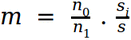 .
.
Note that in the case where the refraction indexes before and after the system are the same : 
In the case of a mirror where the emerging rays propagate against the incident rays direction,  .
.
 Ai position can also be calculated with xi the algebric distance from the vertex of the last optical
surface to Ai.
Ai position can also be calculated with xi the algebric distance from the vertex of the last optical
surface to Ai.
xi is then a function of x, f ( or fi ),
n0, n1, l and li where x is the algebric distance from the vertex of the first optical surface to A, l is the algebric distance from the vertex of the first optical surface to the primary nodal point N and li is the algebric distance from the vertex of the last optical surface to the secondary nodal point Ni.
Sometimes, it can be useful to calculate z and zi which are respectively the algebric distances
FA and FiAi (F and Fi being respectively the front and back focal points) : 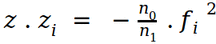 .
.
Aperture
The aperture is supposed to be the only surface of the system stopping light rays. This surface can be in the object space, in the image space or in an intermediate space. In any case, it is possible to define the aperture in the object space: it is the conjugate of the aperture by the sub-system formed with the preceding components and used in the reverse way. Also, it is possible to define the aperture in the image space which is the conjugate of the aperture by the sub-system formed with the following components. The aperture in the object space enables to defines the solid angle inside which the rays are launched from the field(s). The aperture in the image space enables to eventually calculate the Wave Front Error and the associated parameters as well as the diffraction limit of the system. Note that in some cases, vignetting can appear. Indeed, some rays coming from off-xis objects may be stopped by another surface than the said aperture surface. This can affect the aberrations, limit the system resolution and create some shadows on the image. In general, one try to avoid vignetting and this case is not considered in the rest of the tutorial.
An optical system is represented in the pictures below with different aperture positions. Theoretically, the chief rays (chief rays are defined further in this tutorial) coming from different objects (fields) intersect the aperture surface at the same point. This point is the aperture center.
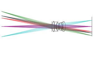
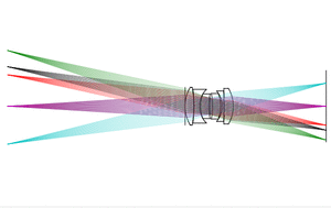 In the left picture, the aperture is defined by the first surface. In the right picture, the aperture is defined by a surface in the middle of the optical system.
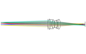
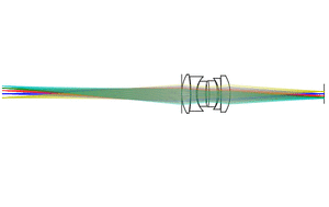 In the left picture, the system is telecentric (aperture at infinity) in the object space as the chief rays in the object space are all parallel. In the right picture, the system is telecentric in the image space as the chief rays in the image space are all parallel.
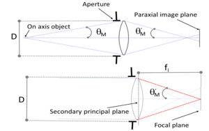 The aperture can be defined in several ways.
It can first be specified by the diameter D of the aperture itself.
It can also be defined by the half aperture angle θM in the object space. θM is the angle with the axis of a ray coming from the on-axis object and passing at the edge of the aperture in the object space (called marginal ray).
θM is often used to specify the aperture of illumination optics. For these systems, θM may be larger than 90°.
The aperture is commonly specified with the numerical aperture in the object space NA.
The aperture can be defined in several ways.
It can first be specified by the diameter D of the aperture itself.
It can also be defined by the half aperture angle θM in the object space. θM is the angle with the axis of a ray coming from the on-axis object and passing at the edge of the aperture in the object space (called marginal ray).
θM is often used to specify the aperture of illumination optics. For these systems, θM may be larger than 90°.
The aperture is commonly specified with the numerical aperture in the object space NA.
 where n is the refraction index in the object space.
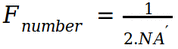
The aperture is also often defined with the F number (common notation: F/N, F#, Fnumber). It is currently the case for many systems as for instance camera lenses.
where n is the refraction index in the object space.
The aperture is also often defined with the F number (common notation: F/N, F#, Fnumber). It is currently the case for many systems as for instance camera lenses.
 .
.
 . is the numerical aperture in the image space (n' is the refraction index in the image space). The larger the aperture, the larger the numerical aperture and the lower the F number.
For optical systems with small aperture and working for objects located at infinity, the F number is approximately the ratio of the focal length fi to the diameter D of the stop surface :
. is the numerical aperture in the image space (n' is the refraction index in the image space). The larger the aperture, the larger the numerical aperture and the lower the F number.
For optical systems with small aperture and working for objects located at infinity, the F number is approximately the ratio of the focal length fi to the diameter D of the stop surface : 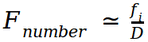 .
.
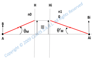 In Gauss conditions, θ'M is the angle with the optical axis of the marginal ray after transmission through the optical system according to the rules of the paraxial conjugation. Therefore, the marginal ray intercepts the on-axis paraxial image on one side and the secondary principal plane on the oher side at the same height than the incident marginal ray on the primary principal plane.
Depth of field
In many cases, an optical system is used for imaging an object in a plane and then detect the image. The detector can be for instance a single detector if the object is almost punctual or it can be a matrix of detectors (matrix of pixels) for recording a scene. This last case corresponds to the type of detectors inside a camera. In practice, the object is not exactly at the theoretical position and the detector is not exactly in the conjugated plane. Ideally, a single detector or a pixel is supposed to detect the image of a punctual object. However, its active area can not be punctual.
It makes then no difference when detecting a punctual image or a spot smaller than the active area. Consequently, in a certain limit, both object point and detector can be located in slightly different planes than the respective oject plane and conjugated plane.
This tolerance is commonly called depth of field or maximum defocus depending if the object or the
detector positioning is considered. Considering a punctual object, the depth of field is the tolerance on the object position enabling to obtain a spot in the theoretical conjugated plane which size is smaller than an authorized value. The maximum defocus is the tolerance on the detector position enabling to obtain a spot size smaller than an authorized value, the object being located at its theoretical position.
In practice, depth of field and maximum defocus are smaller than the above mentionned values as both have to be considered at the same time. These tolerances may be complicated to calculate as the ray propagation is not only defined by paraxial conjugation but involves also aberration and diffraction. Moreover, different criterions can be used to define them depending on the considered application.
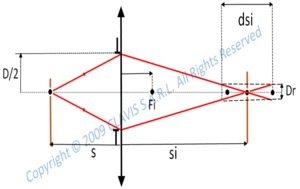
In the following section, depth of field and maximum defocus are only calculated in Gauss conditions without considering any aberration or diffraction effect. Also, the system is a thin lens and the considered distances are algebraic.
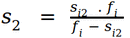
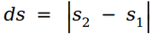
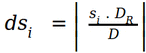
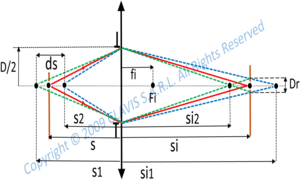 The effective focal length is fi and the aperture diameter is D. Initially, the object and its conjugated are respectively at the distance s and si from the lens. A spot diameter of DR (maximum authorized spot diameter) in the initial conjugated plane is obtained by moving the object in two different positions at the respective distances s1 and s2 from the lens. The corresponding images have then moved and are respectively at the distances si1 and si2 from the lens.
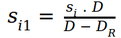 .
and
.
and
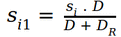 .
According to the paraxial conjugation formulas :
.
According to the paraxial conjugation formulas :
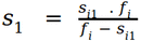 .
and
.
and
 .
Finally, the depth of field is :
.
Finally, the depth of field is :
 .
.
 The depth of focus is :
 .
.
References
"Optique Fondements et applications" - 2004 - author : José-Philippe Perez.
"Optique géométrique Imagerie et instruments" - 2007 - author : Bernard Balland.
"Optique géométrique paraxiale" - Institut doptique théorique et appliquée - 1985 - author : Michel Cagnet.
"Formation des images Aberrations" - Institut doptique théorique et appliquée - 1985 - author : Michel Cagnet.